Improved Denoising Diffusion Probabilistic Models

Alex Nichol, Prafulla Dhariwal

2021 · ICML

Improved Denoising Diffusion Probabilistic Models

Problem

Framing

DDPMs still pay a steep sampling cost and leave likelihood on the table when reverse variances are fixed. This paper closes both gaps with learned variances, a hybrid $\epsilon$ -plus-VLB objective, and a cosine noise schedule. CIFAR-10 reaches FID 2.94, and ImageNet 64 $\times$ 64 reaches 3.53 bits/dim.

Currently Used Methods

Direct antecedents

@DenoisingDiffusionProbabilisticModels2020 — DDPM with fixed reverse variances and $\epsilon$ $ϵ$ -prediction training.
- Limitation in context: weak NLL and thousands of sampling steps.
@DenoisingDiffusionImplicitModels2020 — non-Markovian diffusion sampler for fewer denoising evaluations.
- Limitation in context: speedups are not learned through DDPM variance modeling.
@DeepUnsupervisedLearningusing2015 — early nonequilibrium diffusion likelihood model.
- Limitation in context: far weaker image quality and scale.
@songScoreSDE2020 — continuous-time score modeling with strong likelihoods.
- Limitation in context: this paper targets simple discrete ancestral sampling.

Proposed Method

Architecture

The model keeps the DDPM U-Net and changes the reverse-process parameterization. The network predicts the mean through the usual $\boldsymbol{\epsilon}_{\theta}$ path and learns the variance through an interpolation variable $\mathbf{v}$ between $\beta_t$ and $\tilde{\beta}_t$ .

Verified figure: linear-vs-cosine noise schedules, with latent image strips showing that cosine preserves structure longer while linear becomes pure noise earlier.

Loss / Objective

Training uses a hybrid objective that keeps the DDPM denoising loss dominant while adding a small variational term.

L_{\mathrm{hybrid}} = L_{\mathrm{simple}} + \lambda L_{\mathrm{vlb}}

L_{\mathrm{simple}} = \mathbb{E}_{t,\mathbf{x}_0,\boldsymbol{\epsilon}} \left[ \left\| \boldsymbol{\epsilon} - \boldsymbol{\epsilon}_{\theta}(\mathbf{x}_t,t) \right\|^2 \right]

\Sigma_{\theta}(\mathbf{x}_t,t) = \exp\!\left( \mathbf{v} \log \beta_t + (1-\mathbf{v}) \log \tilde{\beta}_t \right)

Sampling Rule

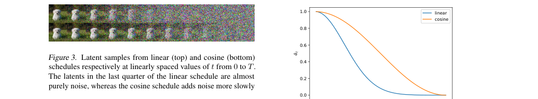
Sampling remains ancestral, with the learned reverse variance and a cosine cumulative-noise schedule.

p_{\theta}(\mathbf{x}_{t-1}\mid \mathbf{x}_t) = \mathcal{N}\!\left( \mathbf{x}_{t-1}; \boldsymbol{\mu}_{\theta}(\mathbf{x}_t,t), \Sigma_{\theta}(\mathbf{x}_t,t) \right)

\bar{\alpha}_t = \frac{f(t)}{f(0)}, \qquad f(t)=\cos^2\!\left( \frac{t/T+s}{1+s} \cdot \frac{\pi}{2} \right)

Training Procedure

Diffusion steps: $T=4000$ .
Hybrid-loss weight: $\lambda=0.001$ .
Optimizer: Adam.
Learning rate: $10^{-4}$ .
EMA decay: $0.9999$ .
Class-conditional ImageNet 64 $\times$ 64 sampling steps: 250.

Evaluation

Datasets

CIFAR-10 unconditional.
ImageNet 64 $\times$ 64 unconditional.
ImageNet 64 $\times$ 64 class-conditional.
ImageNet 256 $\times$ 256 class-conditional.

Metrics

FID.
Inception Score.
NLL in bits/dim.
Precision.
Recall.

Headline results

CIFAR-10 unconditional: FID 2.94.
ImageNet 64 $\times$ 64 unconditional: NLL 3.53 bits/dim.
ImageNet 64 $\times$ 64 class-conditional, small model: FID 19.2, precision 0.66, recall 0.51.
ImageNet 64 $\times$ 64 class-conditional, large model: FID 13.0, precision 0.71, recall 0.54.
ImageNet 256 $\times$ 256 two-stage conditional: 64 $\times$ 64 base FID 2.92 before upsampling.

Table 1: Ablating schedule and objective on ImageNet 64 $\times$ 64.

Iters	T	Schedule	Objective	NLL	FID
200K	1K	linear	$L_{\mathrm{simple}}$	3.99	32.5
200K	4K	linear	$L_{\mathrm{simple}}$	3.77	31.3
200K	4K	linear	$L_{\mathrm{hybrid}}$	3.66	32.2
200K	4K	cosine	$L_{\mathrm{simple}}$	3.68	27.0
200K	4K	cosine	$L_{\mathrm{hybrid}}$	3.62	28.0
200K	4K	cosine	$L_{\mathrm{vlb}}$	3.57	56.7
1.5M	4K	cosine	$L_{\mathrm{hybrid}}$	3.57	19.2
1.5M	4K	cosine	$L_{\mathrm{vlb}}$	3.53	40.1

$Verified results plot: NLL versus evaluation steps on ImageNet 64x64 and CIFAR-10, showing the paper's L_{\mathrm{hybrid}} curves below fixed-variance and DDIM-style baselines, especially at low step counts.$

Ablations

Schedule: cosine beats linear on FID at matched training budget.
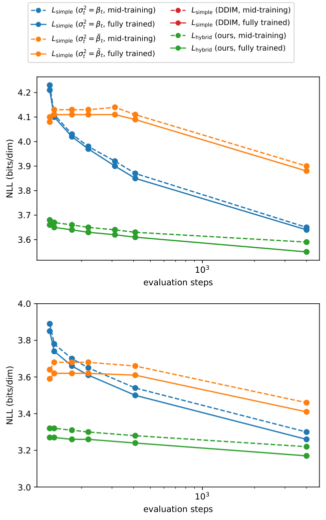
Objective: $L_{\mathrm{vlb}}$ improves NLL but badly hurts FID.
Learned variance: enables far fewer reverse steps with modest quality loss.
Importance-sampled VLB: reduces gradient noise versus direct VLB training.

Method Strengths and Weaknesses

Strengths

Learned variances make 50-step ancestral sampling viable.
Cosine scheduling improves FID over linear scheduling.
Hybrid training improves NLL without collapsing sample quality.
Precision-recall evaluation shows competitive mode coverage.

Weaknesses

Best sampler still needs many sequential denoising steps.
Pure $L_{\mathrm{vlb}}$ training is noisy and unstable.
Best NLL and best FID come from different objectives.
Method still relies on a heavy U-Net backbone.

Suggestions from the authors

Scale model size and training compute further.
Design better low-variance likelihood objectives.
Push sampling to fewer reverse evaluations.
Extend diffusion upsampling to higher resolutions.

Improved Denoising Diffusion Probabilistic Models

Improved Denoising Diffusion Probabilistic Models

Problem

Framing

Currently Used Methods

Direct antecedents

Proposed Method

Architecture

Loss / Objective

Sampling Rule

Training Procedure

Evaluation

Datasets

Metrics

Headline results

Ablations

Method Strengths and Weaknesses

Strengths

Weaknesses

Suggestions from the authors

Links

Prior Papers

Further Papers