Score-Based Generative Modeling through Stochastic Differential Equations

Yang Song, Jascha Sohl-Dickstein, Diederik P. Kingma

2020 · ICLR

Score-Based Generative Modeling through Stochastic Differential Equations

Problem

Framing

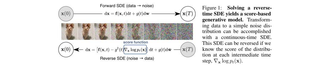
Discrete score models and DDPMs used fixed noise ladders, separate sampler derivations, and no exact likelihood path. The paper unifies them as continuous-time SDEs, then generates with reverse-time SDEs, predictor-corrector sampling, and a probability-flow ODE. On CIFAR-10, it reports FID 2.20 and 2.99 bits/dim.

Currently Used Methods

Foundational

@DeepUnsupervisedLearningusing2015 — annealed score matching with Langevin dynamics over discrete noise scales.
- Limitation in context: fixed noise ladder, with no continuous-time formulation.
@DenoisingDiffusionProbabilisticModels2020 — discrete diffusion with a learned reverse Markov chain.
- Limitation in context: tied to one discretization, without exact ODE likelihoods.
@dinhNVP2017 — invertible flows with exact likelihood computation.
- Limitation in context: weaker image sample quality than score-SDE models.
Improved Techniques for Training Score-Based Generative Models — stronger score-network training and sampling heuristics.
- Limitation in context: still discrete in noise scale and sampler design.

Proposed Method

Architecture

The framework has three parts: a forward SDE, a time-conditioned score network $\mathbf{s}_{\theta}(\mathbf{x}, t)$ , and a reverse-time solver. Experiments use DDPM backbones and NCSN++, which adds FIR up/downsampling, $1/\sqrt{2}$ skip rescaling, BigGAN-style residual blocks, and progressive input/output paths.

Overview diagram: data are diffused to noise by a forward SDE, and a learned score field drives the reverse SDE from noise back to data.

Loss / Objective

Training fits the time-dependent score along SDE marginals.

\min_{\theta} \; \mathbb{E}_{t \sim \mathrm{Unif}(0,T)} \left[ \lambda(t) \, \mathbb{E}_{\mathbf{x}(0) \sim p_0} \, \mathbb{E}_{\mathbf{x}(t) \sim p_{0t}(\mathbf{x}(t) \mid \mathbf{x}(0))} \left[ \left\| \mathbf{s}_{\theta}(\mathbf{x}(t), t) - \nabla_{\mathbf{x}(t)} \log p_{0t}(\mathbf{x}(t) \mid \mathbf{x}(0)) \right\|_2^2 \right] \right]

Sampling Rule / Algorithm

Generation solves the reverse-time SDE; the paper also uses a deterministic probability-flow ODE.

\mathrm{d}\mathbf{x} = \left[ \mathbf{f}(\mathbf{x}, t) - g(t)^2 \nabla_{\mathbf{x}} \log p_t(\mathbf{x}) \right] \, \mathrm{d}t + g(t) \, \mathrm{d}\bar{\mathbf{w}}

\mathrm{d}\mathbf{x} = \left[ \mathbf{f}(\mathbf{x}, t) - \frac{1}{2} g(t)^2 \nabla_{\mathbf{x}} \log p_t(\mathbf{x}) \right] \, \mathrm{d}t

Training Procedure

Noise scales for discrete counterparts: 1000.
Default training length: 1.3M iterations.
Checkpoints: every 50k iterations.
Batch size: 128 on CIFAR-10.
Batch size: 64 on LSUN.
CelebA-HQ 1024 $\times$ 1024 batch size: 8.
CelebA-HQ 1024 $\times$ 1024 EMA: 0.9999.

Evaluation

Datasets

CIFAR-10, 32 $\times$ 32.
CelebA, 64 $\times$ 64.
LSUN bedroom, 256 $\times$ 256.
LSUN church outdoor, 256 $\times$ 256.
CelebA-HQ, 256 $\times$ 256 and 1024 $\times$ 1024.

Metrics

FID.
Inception Score.
Test NLL / bits per dimension.

Headline results

CIFAR-10 unconditional: FID 2.20, IS 9.89.
CIFAR-10 sub-VP ODE likelihood: 2.99 bits/dim.
CIFAR-10 VE SDE + NCSN++ + PC: FID 2.45.
CIFAR-10 VP or sub-VP continuous model: FID 2.41.
CelebA-HQ 1024 $\times$ 1024: high-fidelity score-model samples.

Table 1: CIFAR-10 FID for reverse-time samplers under VE-SDE and VP-SDE parameterizations.

Predictor	VE P1000	VE P2000	VE C2000	VE PC1000	VP P1000	VP P2000	VP C2000	VP PC1000
ancestral sampling	4.98 $\pm$ .06	4.88 $\pm$ .06		3.62 $\pm$ .03	3.24 $\pm$ .02	3.24 $\pm$ .02		3.21 $\pm$ .02
reverse diffusion	4.79 $\pm$ .07	4.74 $\pm$ .08	20.43 $\pm$ .07	3.60 $\pm$ .02	3.21 $\pm$ .02	3.19 $\pm$ .02	19.06 $\pm$ .06	3.18 $\pm$ .01
probability flow	15.41 $\pm$ .15	10.54 $\pm$ .08		3.51 $\pm$ .04	3.59 $\pm$ .04	3.23 $\pm$ .03		3.06 $\pm$ .03

Ablations

Sampler choice: predictor-corrector beats predictor-only at matched score evaluations.
ODE solver: probability flow stays competitive while enabling likelihood computation.
Architecture components: FIR, skip rescaling, BigGAN blocks, and progressive paths improve VE-SDE FID.
EMA rate: larger EMA materially improves VE-SDE performance.

Method Strengths and Weaknesses

Strengths

Unifies SMLD and DDPM as VE and VP SDE discretizations.
Adds exact likelihoods through the probability-flow ODE.
Predictor-corrector sampling improves FID at similar evaluation budgets.
Reaches CIFAR-10 FID 2.20 with 2.99 bits/dim in one framework.

Weaknesses

High-quality sampling still needs many score evaluations.
Continuous denoising objective needs tractable perturbation kernels.
Best results rely on substantial architecture tuning beyond the SDE abstraction.
1024 $\times$ 1024 training uses batch size 8 and very long runs.

Suggestions from the authors

Reduce the sampling cost of reverse-time solvers.
Extend the framework to general SDEs with state-dependent diffusion.
Broaden conditional generation to harder inverse problems.
Improve architectures and objectives for better likelihood and FID.

Score-Based Generative Modeling through Stochastic Differential Equations

Score-Based Generative Modeling through Stochastic Differential Equations

Problem

Framing

Currently Used Methods

Foundational

Proposed Method

Architecture

Loss / Objective

Sampling Rule / Algorithm

Training Procedure

Evaluation

Datasets

Metrics

Headline results

Ablations

Method Strengths and Weaknesses

Strengths

Weaknesses

Suggestions from the authors

Links

Prior Papers

Further Papers