Deep Unsupervised Learning using Nonequilibrium Thermodynamics
Deep Unsupervised Learning using Nonequilibrium Thermodynamics
Problem
Framing
Generative models had not combined normalized likelihood, exact ancestral sampling, and easy conditional manipulation in one stochastic framework. The paper closes that gap by diffusing data to a tractable terminal law, then learning only local reverse kernels. On dead leaves it reports bits/pixel.
Currently Used Methods
Foundational
- @hintonDeepBeliefNets2006 — greedy layerwise training for deep probabilistic models.
- Limitation in context: no stochastic diffusion path with local reverse-step targets.
- @kingmaVAE2013 — amortized latent-variable likelihood modeling.
- Limitation in context: depends on approximate inference, not reversible corruption dynamics.
- @goodfellowGAN2014 — adversarial generation with sharp samples.
- Limitation in context: lacks normalized likelihood and cheap state-probability evaluation.
- @dinhNVP2017 — invertible exact-likelihood transformations.
- Limitation in context: uses deterministic bijections, not stochastic diffusion transitions.
Proposed Method
Architecture
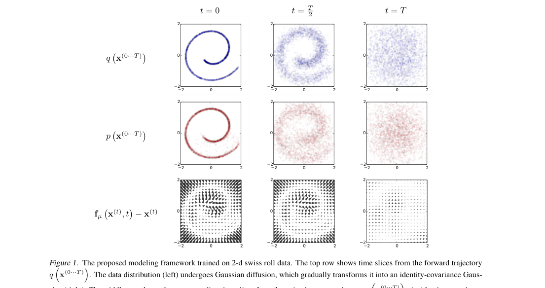
The model defines a forward diffusion chain and a learned reverse chain . For images, the reverse model predicts per-step mean and covariance from multiscale convolutions followed by several convolutions. Time enters through learned bump-function coefficients over .
Loss / Objective
Training maximizes a variational lower bound on log likelihood.
Sampling Rule / Algorithm
Sampling starts from the tractable terminal distribution and applies learned reverse kernels for steps.
Training Procedure
- Swiss roll: Gaussian steps.
- Binary heartbeat: binomial steps.
- Images: .
- Bark: .
- Optimizer: RMSprop.
- Swiss roll MLP hidden width: .
- Heartbeat MLP: hidden layers, units each.
Evaluation
Datasets
- Swiss roll
- Binary heartbeat sequences
- MNIST
- CIFAR-10
- Bark textures
- Dead leaves
Metrics
- Variational lower bound
- Improvement over null model
- Bits
- Bits per sequence
- Bits per pixel
Headline results
- Swiss roll: bits, bits.
- Binary heartbeat: bits/seq; true process bits/seq.
- Dead leaves: bits/pixel.
- CIFAR-10: posterior denoising and unconditional samples are shown.
- MNIST: true ancestral samples are shown.
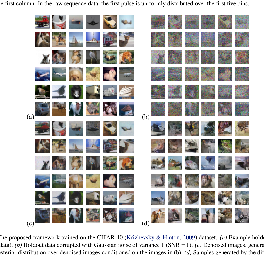
Table 1: Log-likelihood summary across datasets.
| Dataset | K | K - Lnull |
|---|---|---|
| Swiss Roll | 2.35 bits | 6.45 bits |
| Binary Heartbeat | -2.414 bits/seq. | 2.676 bits/seq. |
| MNIST | 82.90 bits | 136.7 bits |
| CIFAR-10 | 4.51 bits/pixel | 0.59 bits/pixel |
| Dead Leaves | ||
| MCGSM | 1.244 bits/pixel | |
| Diffusion probabilistic model | 1.184 bits/pixel | 0.53 bits/pixel |
Ablations
- Diffusion length : larger makes each reverse step easier to estimate.
- Forward kernel family: Gaussian and binomial diffusions use one training framework.
- Noise schedule: likelihood depends on the hand-chosen diffusion-rate schedule.
- Task type: the same formulation covers continuous images and binary sequences.
Method Strengths and Weaknesses
Strengths
- Reduces density learning to local reverse-step estimation.
- Supports exact ancestral sampling from a normalized model.
- Handles Gaussian images and binomial sequences in one framework.
- Reports bits/pixel on dead leaves, close to MCGSM's .
Weaknesses
- Sampling cost scales linearly with the full horizon .
- Image backbone predates U-Net-style denoisers.
- CIFAR-10 evaluation is qualitative.
- Performance depends on hand-designed diffusion schedules.
Suggestions from the authors
- Learn diffusion-rate schedules instead of fixing them.
- Extend the framework to richer diffusion kernels.
- Use distribution multiplication for conditional inference.
- Scale reverse models for long diffusion chains.
Links
Prior Papers
- @hintonDeepBeliefNets2006 — early deep probabilistic training background for tractable generative modeling.
- @kingmaVAE2013 — variational likelihood modeling targets the same density-estimation problem.
- @goodfellowGAN2014 — contrasting route to sharp generation without normalized likelihood.
- @dinhNVP2017 — exact-likelihood generative modeling via invertible transformations.
Further Papers
- @DenoisingDiffusionProbabilisticModels2020 — turns this thermodynamic formulation into the modern denoising objective.
- @DenoisingDiffusionImplicitModels2020 — accelerates sampling within the same diffusion lineage.
- @ClassifierFreeDiffusionGuidance2022 — adds strong conditional control to diffusion generation.
- @nicholImprovedDDPM2021 — improves likelihoods and sampling efficiency for DDPM-style models.
- @songScoreSDE2020 — recasts diffusion generation as continuous-time score dynamics.