Continuous control with deep reinforcement learning
Continuous control with deep reinforcement learning
Problem
Framing
Deep RL had not made off-policy value learning work in continuous action spaces with large neural function approximators. The paper closes this gap by combining deterministic policy gradients with replay, target networks, and batch normalization, then learning directly from pixels on many MuJoCo tasks and Torcs.
Currently Used Methods
Foundational
- @mnihDQN2015 — replay and target networks stabilize deep off-policy value learning.
- Limitation in context: argmax over continuous actions is intractable.
- @schulmanTRPO2015 — constrained stochastic policy optimization for continuous control.
- Limitation in context: on-policy updates waste data and avoid off-policy critics.
- Deterministic Policy Gradient — actor update through for continuous actions.
- Limitation in context: naive deep implementations are unstable on hard domains.
- NFQCA — neural fitted Q actor-critic with minibatch updates.
- Limitation in context: does not stabilize large-scale pixel-based control.
- Stochastic Value Gradients — critic-based policy learning with stochastic policies.
- Limitation in context: this paper targets simpler deterministic actors with replay.
Proposed Method
Architecture
DDPG uses an actor and critic , each with target copies. For low-dimensional states, both networks use two hidden layers with 400 and 300 units; the critic injects the action at the second hidden layer, and batch normalization is applied to state inputs and intermediate layers.
Loss / Objective
The critic minimizes the Bellman residual with a target-network bootstrap:
Sampling Rule / Algorithm
The actor follows the deterministic policy gradient estimated from replay-buffer states:
Target networks are updated by soft averaging:
Training Procedure
- Replay buffer: transitions.
- Minibatch size: .
- Discount: .
- Soft target rate: .
- Actor learning rate: .
- Critic learning rate: .
- Critic weight decay: .
- Exploration: Ornstein-Uhlenbeck noise.
- Optimizer: Adam.
Evaluation
Datasets
- Continuous-control benchmarks in MuJoCo.
- Both low-dimensional state input and pixel input settings.
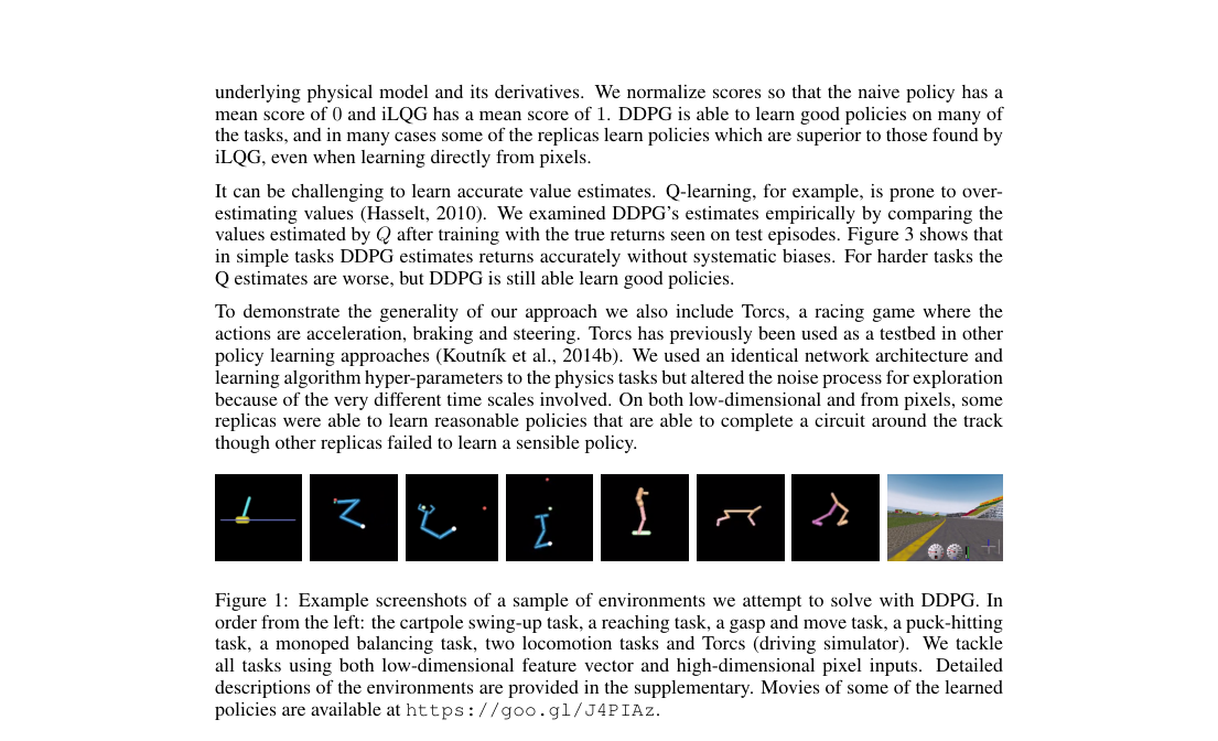
- Torcs for vision-based driving.
Metrics
- Normalized reward: random policy , planner .
- Torcs raw return.
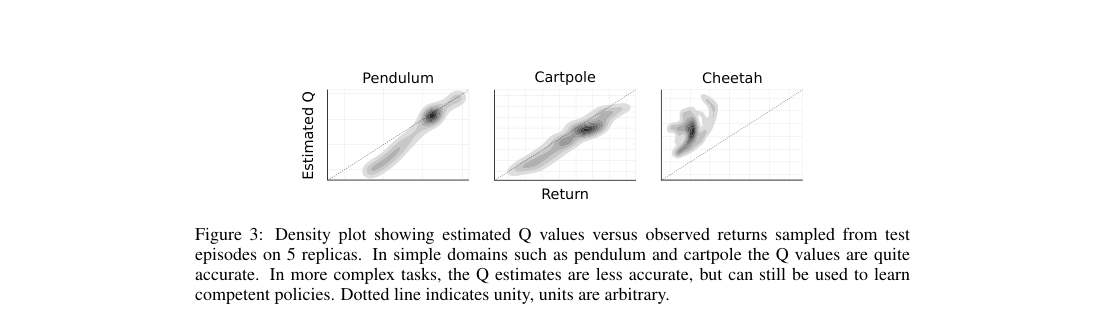
- Estimated versus realized return diagnostics.
Headline results
- blockworld: lowd avg, best; pixels avg, best.
- cartpoleBalance: lowd avg, best; pixels avg, best.
- cheetah: lowd avg, best; pixels avg, best.
- pendulum: lowd avg, best; pixels avg, best.
- walker2d: lowd avg, best; pixels avg, best.
Table 1: Performance after training for at most 2.5 million steps; random policy is 0 and planner is 1 (except Torcs).
| Rav,lowd | Rbest,lowd | Rav,pix | Rbest,pix | Rav,cntrl |
|---|---|---|---|---|
| 1.156 | 1.511 | 0.466 | 1.299 | -0.080 |
| 0.340 | 0.705 | 0.889 | 2.225 | -0.139 |
| 0.303 | 1.735 | 0.176 | 0.688 | 0.125 |
| 0.400 | 0.978 | -0.285 | 0.119 | -0.045 |
| 0.938 | 1.336 | 1.096 | 1.258 | 0.343 |
| 0.844 | 1.115 | 0.482 | 1.138 | 0.244 |
| 0.951 | 1.000 | 0.335 | 0.996 | -0.468 |
| 0.549 | 0.900 | 0.188 | 0.323 | 0.197 |
| 0.272 | 0.719 | 0.195 | 0.642 | 0.143 |
| 0.736 | 0.946 | 0.412 | 0.427 | 0.583 |
| 0.903 | 1.206 | 0.457 | 0.792 | -0.008 |
| 0.849 | 1.021 | 0.693 | 0.981 | 0.259 |
| 0.924 | 0.996 | 0.872 | 0.943 | 0.290 |
| 0.954 | 1.000 | 0.827 | 0.995 | 0.620 |
| 0.655 | 0.972 | 0.406 | 0.790 | 0.461 |
| 0.618 | 0.937 | 0.082 | 0.791 | 0.557 |
| 1.311 | 1.990 | 1.204 | 1.431 | -0.031 |
| 0.676 | 0.936 | 0.112 | 0.924 | 0.078 |
| 0.416 | 0.722 | 0.234 | 0.672 | 0.198 |
| 0.474 | 0.936 | 0.480 | 0.644 | 0.416 |
| 0.946 | 1.021 | 0.663 | 1.055 | 0.099 |
| 0.720 | 0.987 | 0.194 | 0.878 | 0.231 |
| 0.585 | 0.943 | 0.453 | 0.922 | 0.204 |
| 0.467 | 0.739 | 0.374 | 0.735 | -0.046 |
| 0.981 | 1.102 | 1.000 | 1.083 | 1.010 |
| 0.705 | 1.573 | 0.944 | 1.476 | 0.393 |
Ablations
- Target networks: crucial for stable learning curves.
- Batch normalization: improves actor-critic training across tasks.
- Pixel input: remains competitive with low-dimensional control on several tasks.
- Q calibration: accurate on pendulum and cartpole, worse on cheetah but still useful.
Method Strengths and Weaknesses
Strengths
- Extends replay-buffer off-policy learning to continuous actions.
- Learns directly from pixels across many continuous-control tasks.
- Soft target updates materially improve stability.
- Beats or matches planner-normalized score on several domains.
Weaknesses
- Training remains fragile; some replicas fail on hard tasks.
- Q estimates degrade on complex domains like cheetah.
- Requires many environment steps: up to million.
- Performance variance is large between average and best runs.
Suggestions from the authors
- Study why value estimates remain useful despite poor calibration on hard tasks.
- Improve stability and reproducibility across random seeds.
- Extend pixel-based continuous control to broader real-world domains.
- Analyze stronger exploration processes for tasks with long time scales.
Links
Prior Papers
- @mnihDQN2015 — contributes replay and target-network ideas that DDPG adapts to actor-critic control.
- @schulmanTRPO2015 — another early deep continuous-control baseline with a contrasting on-policy optimization strategy.
Further Papers
- @mnihA3C_2016 — another major deep RL control method from the same period, useful as an on-policy contrast.
- @hafnerDreamerV1_2019 — extends continuous-control learning with latent world models and actor-critic updates.
- @schulmanTRPO2015 — remains a close policy-optimization counterpart for continuous control.