Soft Actor-Critic: Off-Policy Maximum Entropy Deep Reinforcement Learning with a Stochastic Actor

Tuomas Haarnoja, Aurick Zhou, Pieter Abbeel, Sergey Levine

2018 · ICML

Soft Actor-Critic: Off-Policy Maximum Entropy Deep Reinforcement Learning with a Stochastic Actor

Problem

Framing

Deep RL in continuous control faced a bad tradeoff: on-policy methods were stable but sample-inefficient, while off-policy actor-critics were brittle. SAC closes it by optimizing a maximum-entropy objective with an off-policy stochastic actor and clipped double-Q updates, yielding stable gains on Hopper, Walker2d, HalfCheetah, Ant, and Humanoid.

Currently Used Methods

Foundational

@schulmanTRPO2015 — trust-region policy gradients for stable continuous-control updates.
- Limitation in context: on-policy sampling makes learning far less efficient.
@lillicrapDDPG2015 — deterministic off-policy actor-critic for continuous actions.
- Limitation in context: unstable optimization and weak exploration on hard tasks.
@mnihA3C_2016 — asynchronous on-policy training that improves robustness.
- Limitation in context: still spends too many environment interactions.
"Trust Region Path Consistency Learning" — maximum-entropy RL with path-consistency constraints.
- Limitation in context: weaker performance on the hardest MuJoCo tasks.

Proposed Method

Architecture

SAC uses a stochastic Gaussian policy, two soft Q-functions, one soft value network, and a target value network. The policy samples an unconstrained Gaussian action and squashes it with $\tanh$ to satisfy action bounds.

\mathbf{a}_t = \tanh\left(\boldsymbol{\mu}_\phi(\mathbf{s}_t) + \boldsymbol{\sigma}_\phi(\mathbf{s}_t) \odot \boldsymbol{\epsilon}_t\right), \quad \boldsymbol{\epsilon}_t \sim \mathcal{N}(\mathbf{0}, \mathbf{I})

Loss / Objective

SAC maximizes reward plus entropy under the discounted occupancy measure.

J(\pi) = \sum_{t=0}^{T} \mathbb{E}_{(\mathbf{s}_t,\mathbf{a}_t) \sim \rho_\pi}\left[r(\mathbf{s}_t,\mathbf{a}_t) + \alpha \, \mathcal{H}\big(\pi(\cdot \mid \mathbf{s}_t)\big)\right]

The practical critic, value, and actor losses are:

J_Q(\boldsymbol{\theta}) = \mathbb{E}_{(\mathbf{s}_t,\mathbf{a}_t) \sim \mathcal{D}} \left[\frac{1}{2}\left(Q_{\boldsymbol{\theta}}(\mathbf{s}_t,\mathbf{a}_t) - \hat{Q}(\mathbf{s}_t,\mathbf{a}_t)\right)^2\right]

\hat{Q}(\mathbf{s}_t,\mathbf{a}_t) = r(\mathbf{s}_t,\mathbf{a}_t) + \gamma \, V_{\bar{\boldsymbol{\psi}}}(\mathbf{s}_{t+1})

J_V(\boldsymbol{\psi}) = \mathbb{E}_{\mathbf{s}_t \sim \mathcal{D}}\left[\frac{1}{2}\left(V_{\boldsymbol{\psi}}(\mathbf{s}_t) - \mathbb{E}_{\mathbf{a}_t \sim \pi_\phi}\left[\min_{j=1,2} Q_{\boldsymbol{\theta}_j}(\mathbf{s}_t,\mathbf{a}_t) - \log \pi_\phi(\mathbf{a}_t \mid \mathbf{s}_t)\right]\right)^2\right]

J_\pi(\boldsymbol{\phi}) = \mathbb{E}_{\mathbf{s}_t \sim \mathcal{D}, \, \boldsymbol{\epsilon}_t \sim \mathcal{N}}\left[\log \pi_\phi\big(f_\phi(\boldsymbol{\epsilon}_t;\mathbf{s}_t) \mid \mathbf{s}_t\big) - \min_{j=1,2} Q_{\boldsymbol{\theta}_j}\big(\mathbf{s}_t, f_\phi(\boldsymbol{\epsilon}_t;\mathbf{s}_t)\big)\right]

Sampling Rule / Algorithm

Training alternates soft policy evaluation, reparameterized actor updates, and Polyak target updates.

\bar{\boldsymbol{\psi}} \leftarrow \tau \, \boldsymbol{\psi} + (1-\tau) \, \bar{\boldsymbol{\psi}}

Training Procedure

Optimizer: Adam.
Learning rate: $3 \times 10^{-4}$ .
Discount: $\gamma = 0.99$ .
Replay buffer size: $10^6$ .
Target smoothing coefficient: $\tau = 0.005$ .
Target update interval: 1 gradient step.
Hidden units per layer: 300.
Minibatch size: 256.
Gradient steps per environment step: 1.

Evaluation

Datasets

Hopper-v1
Walker2d-v1
HalfCheetah-v1
Ant-v1
Humanoid-v1
Humanoid (rllab)

Metrics

Average return versus environment steps.
Final control performance on continuous-control benchmarks.
Stability across random seeds.

Headline results

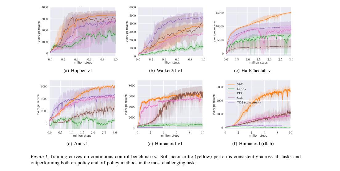
Hopper-v1: SAC reaches about 3.3k average return by 1M steps.
Walker2d-v1: SAC reaches about 3.7k by 1M steps, below concurrent TD3 early.
HalfCheetah-v1: SAC reaches about 15k by 3M steps, best among compared methods.
Ant-v1: SAC reaches about 6k by 3M steps, ahead of PPO, SQL, and DDPG.
Humanoid-v1 / Humanoid (rllab): SAC is the only compared method with strong sustained gains on the hardest tasks.

Training curves across six continuous-control benchmarks; SAC is the orange curve and leads on the hardest tasks.

Ablations

Evaluation mode: deterministic mean-action evaluation scores above stochastic evaluation.
Reward scale: intermediate values work best; too small or too large hurts return.
Target smoothing coefficient $\tau$ : very small $\tau$ slows learning, very large $\tau$ destabilizes it.

Table 1: Sensitivity of SAC on Ant-v1 to evaluation mode, reward scale, and target smoothing coefficient.

Setting	Observation
Deterministic vs stochastic evaluation	Deterministic evaluation finishes higher.
Reward scale $\{1, 3, 10, 30, 100\}$	Mid-range scales perform best; scale 1 underperforms.
Target smoothing coefficient $\tau \in \{0.0001, 0.001, 0.01, 0.1\}$	$0.001$ and $0.01$ work well; $0.1$ collapses.

Method Strengths and Weaknesses

Strengths

Off-policy updates cut sample cost relative to TRPO-class methods.
Stochastic actor improves exploration over deterministic DDPG-style control.
Clipped double-Q and target smoothing improve stability across seeds.
Strongest gains appear on Ant and both Humanoid benchmarks.

Weaknesses

Performance depends strongly on reward scale.
Performance depends on target smoothing coefficient $\tau$ .
Walker2d learning lags concurrent TD3 early in training.
This version needs an extra learned value network, adding complexity.

Suggestions from the authors

Remove sensitivity to reward scaling.
Reduce hyperparameter tuning across environments.
Extend the method to harder real-world robotic tasks.
Study simpler updates without losing SAC stability.

Soft Actor-Critic: Off-Policy Maximum Entropy Deep Reinforcement Learning with a Stochastic Actor

Soft Actor-Critic: Off-Policy Maximum Entropy Deep Reinforcement Learning with a Stochastic Actor

Problem

Framing

Currently Used Methods

Foundational

Proposed Method

Architecture

Loss / Objective

Sampling Rule / Algorithm

Training Procedure

Evaluation

Datasets

Metrics

Headline results

Ablations

Method Strengths and Weaknesses

Strengths

Weaknesses

Suggestions from the authors

Links

Prior Papers

Further Papers