Stochastic Interpolants: A Unifying Framework for Flows and Diffusions

Problem

Framing

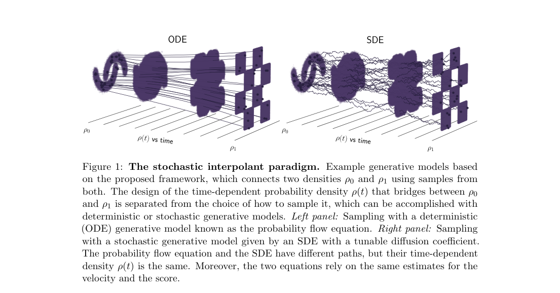
Flow matching and score-based diffusion gave separate recipes for ODE and SDE generative transport, with different objectives and likelihood guarantees. This paper unifies them with stochastic interpolants: design any finite-time bridge $\rho(t)$ between $\rho_0$ and $\rho_1$, then sample it with either a probability-flow ODE or an SDE using quadratic regression losses.

Currently Used Methods

Foundational

• @DenoisingDiffusionProbabilisticModels2020 — discrete diffusion with denoising training for generative sampling.
  • Limitation in context: fixed Gaussian base and effectively long-time corruption process.
• @songScoreSDE2020 — score-based SDEs with reverse-time stochastic sampling.
  • Limitation in context: bridges data to Gaussian, not arbitrary endpoint densities.
• @lipmanFlowMatching2022 — regression of vector fields along prescribed probability paths.
  • Limitation in context: focuses on deterministic transport, not unified stochastic sampling.
• @liuRectifiedFlow2022 — learns straighter ODE trajectories for fast generation.
  • Limitation in context: does not furnish the score-controlled SDE view.
• @karrasEDM2022 — careful diffusion design and ODE/SDE samplers for image generation.
  • Limitation in context: remains tied to Gaussian-noising diffusion parameterizations.

Proposed Method

Architecture

The core object is the interpolant

It separates bridge design from sampler choice. The same learned velocity and score define either deterministic probability flow or stochastic dynamics.

Loss / Objective

Velocity and score are learned by least-squares regression on interpolant samples.

Sampling Rule / Algorithm

The same bridge density admits both a probability-flow ODE and a forward SDE with tunable diffusion $\epsilon(t)$.

Training Procedure

• Image backbone: U-Net from @DenoisingDiffusionProbabilisticModels2020.
• ImageNet $32 \times 32$: batch size $512$.
• Flowers $128 \times 128$: batch size $64$.
• Flowers mirror $128 \times 128$: batch size $64$.
• Optimization target: learn $b$, $v$, $s$, or $\eta$ with gradient steps $N_g$.
• 2D experiments: MLP depth $4$, width $512$, training iterations $7000$.

Evaluation

Datasets

• 2D checkerboard density.
• 128D Gaussian mixtures.
• Oxford Flowers $128 \times 128$.
• ImageNet $32 \times 32$.

Metrics

• $\mathrm{KL}(\rho_1 \| \hat{\rho}(1))$ for synthetic densities.
• Absolute log-density error statistics for 2D studies.
• FID for image generation.

Headline results

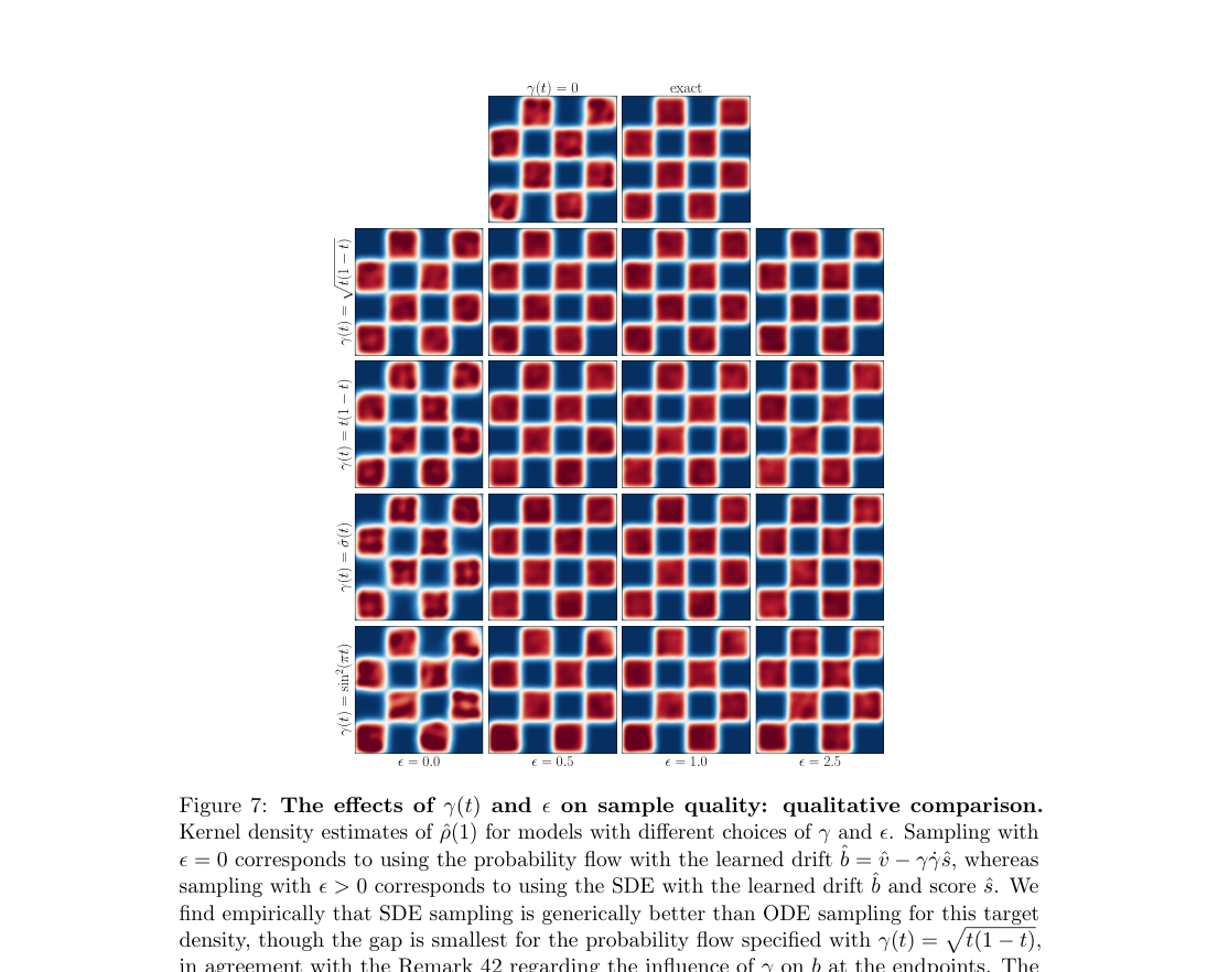
• 2D checkerboard: SDE sampling beats probability flow across most $\gamma(t), \epsilon$ choices.
• 2D checkerboard: best ODE occurs near $\gamma(t)=\sqrt{t(1-t)}$.
• 128D Gaussian mixtures: best quantitative performance comes from learning $b$ and $\eta$.
• Oxford Flowers $128 \times 128$: framework scales to high-dimensional image synthesis.
• ImageNet $32 \times 32$: appendix reports a full image-generation configuration.

Ablations

• Latent-noise schedule $\gamma(t)$: changes intermediate density geometry and final sample quality.
• Diffusion level $\epsilon$: moderate stochasticity improves over pure probability flow.
• Learned targets $(b,s)$ vs $(b,\eta)$ vs $(v,s)$ vs $(v,\eta)$: $(b,\eta)$ performs best.
• Interpolant family: some linear paths create spurious intermediate modes; better $\gamma(t)$ avoids them.

Method Strengths and Weaknesses

Strengths

• One bridge density supports both ODE and SDE generators.
• Training reduces to simple quadratic regression objectives.
• Handles arbitrary endpoint densities, not only Gaussian bases.
• Derives explicit likelihood-control bounds for stochastic models.

Weaknesses

• Deterministic likelihood control is stricter than stochastic likelihood control.
• Sample quality depends strongly on hand-designed $\gamma(t)$ and $\epsilon$.
• Main quantitative evidence centers on synthetic densities more than standard image benchmarks.
• Theory is broad, but practical recipes remain specialized to selected interpolant families.

Suggestions from the authors

• Optimize over interpolants to recover Schrödinger bridges more directly.
• Characterize when deterministic transport can match stochastic sample quality.
• Develop better interpolant designs for high-dimensional data.
• Improve practical likelihood and cross-entropy estimation procedures.

Links

Prior Papers

• @lipmanFlowMatching2022 — flow matching is the closest deterministic antecedent; this paper extends it to shared ODE/SDE bridges.
• @liuRectifiedFlow2022 — rectified flow is analyzed as a related ODE reformulation within the interpolant framework.
• @songScoreSDE2020 — score-based SDE diffusion appears as a special one-sided interpolant after reparameterization.
• @DenoisingDiffusionProbabilisticModels2020 — the image experiments reuse its U-Net backbone and connect denoising objectives to interpolant scores.

Further Papers

• @songConsistencyModels2023 — studies faster generative transport and can be read as a descendant of ODE/SDE unification ideas.
• @peeblesDiT2022 — later diffusion architecture work can inherit this paper's bridge-versus-sampler separation.
• @ClassifierFreeDiffusionGuidance2022 — downstream diffusion sampling methods operate on the same learned score-driven generative setting.