Consistency Models
Consistency Models
Problem
Framing
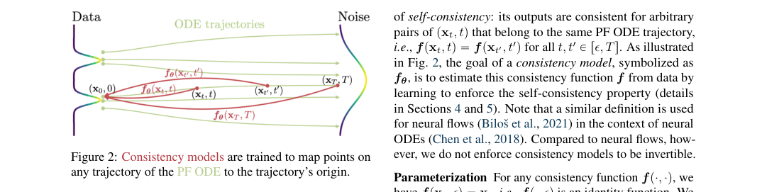
Diffusion models deliver strong sample quality but need 10–2000 denoising steps at inference. This paper replaces iterative denoising with a self-consistent map from any PF-ODE state to the trajectory origin, enabling one-step generation while retaining multistep refinement. One-step FID reaches 3.55 on CIFAR-10 and 6.20 on ImageNet .
Currently Used Methods
Direct antecedents
- @songScoreSDE2020 — score-SDE generation via reverse-time dynamics and PF ODEs.
- Limitation in context: still needs many solver steps for high-quality sampling.
- @karrasEDM2022 — improved diffusion design and Heun-based fast samplers.
- Limitation in context: fast samplers still remain iterative, not one-step.
- @DenoisingDiffusionImplicitModels2020 — deterministic diffusion sampling with fewer evaluations.
- Limitation in context: sample quality still degrades at very low NFE.
- @nicholImprovedDDPM2021 — learned-variance diffusion with fewer sampling steps.
- Limitation in context: reduced-step diffusion is still slower than direct generation.
- @DenoisingDiffusionProbabilisticModels2020 — denoising diffusion training and ancestral sampling.
- Limitation in context: iterative reverse chain makes inference expensive.
Proposed Method
Architecture
The model learns , a map from any PF-ODE point to the same origin .It enforces the boundary condition with a skip-style parameterization
where and . Experiments reuse EDM backbones with modified skip connections.
Loss / Objective
Distillation trains neighboring PF-ODE states to produce identical outputs.
Standalone training replaces the solver pair with two Gaussian-corrupted views of the same data point.
Sampling Rule
One-step generation evaluates the model once at terminal noise. Multistep sampling alternates noise injection and consistency projection.
For distillation, adjacent PF-ODE states are linked by a one-step solver update.
Training Procedure
- PF-ODE horizon: , .
- CIFAR-10: learning rate , batch size 512, for CD.
- ImageNet : learning rate , batch size 2048, for CD.
- LSUN : learning rate , batch size 2048, for CD.
- ODE solver for CD: Heun.
- EMA decay: 0.9999 on CIFAR-10; 0.999943 on ImageNet and LSUN.
- CT schedules: ; on CIFAR-10 and LSUN, on ImageNet; or .
Evaluation
Datasets
- CIFAR-10
- ImageNet
- LSUN Bedroom
- LSUN Cat
Metrics
- FID
- Inception Score (CIFAR-10)
- Precision
- Recall
Headline results
- CIFAR-10, one-step CD: FID 3.55, IS 9.93.
- CIFAR-10, two-step CD: FID 2.93, IS 9.85.
- ImageNet , one-step CD: FID 6.20.
- ImageNet , two-step CD: FID 4.70.
- CT beats prior one-step non-adversarial generators on CIFAR-10, ImageNet , and LSUN.
Ablations
- Metric in CD: LPIPS beats and on CIFAR-10.
- Solver in CD: Heun beats Euler at matched .
- Distillation steps : larger helps until diminishing returns.
- CT schedules: adaptive and accelerate convergence.
Results figure
Figure 3 studies training choices on CIFAR-10: metric, solver, discretization steps, and adaptive schedules.
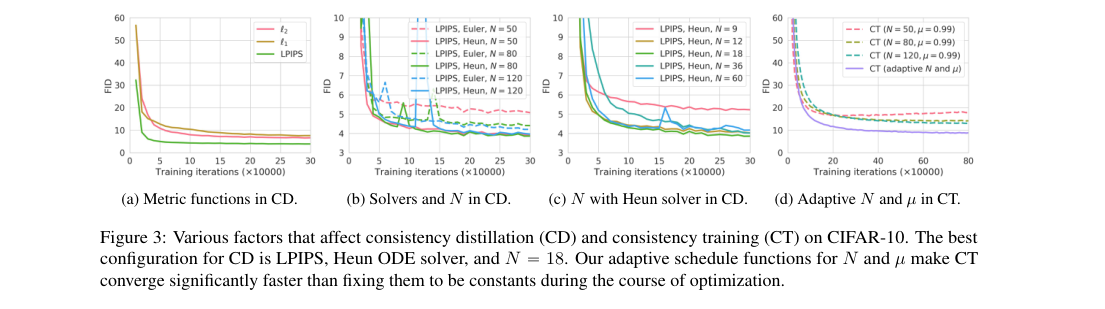
Table 1: Hyperparameters used for training CD and CT models
| Hyperparameter | CIFAR-10 CD | CIFAR-10 CT | ImageNet 64 × 64 CD | ImageNet 64 × 64 CT | LSUN 256 × 256 CD | LSUN 256 × 256 CT |
|---|---|---|---|---|---|---|
| Learning rate | 4e-4 | 4e-4 | 8e-6 | 8e-6 | 1e-5 | 1e-5 |
| Batch size | 512 | 512 | 2048 | 2048 | 2048 | 2048 |
| 0 | 0.95 | 0.95 | ||||
| 0.9 | 0.95 | 0.95 | ||||
| 2 | 2 | 2 | ||||
| 150 | 200 | 150 | ||||
| 18 | 40 | 40 | ||||
| ODE solver | Heun | Heun | Heun | |||
| EMA decay rate | 0.9999 | 0.9999 | 0.999943 | 0.999943 | 0.999943 | 0.999943 |
| Training iterations | 800k | 800k | 600k | 800k | 600k | 1000k |
| Mixed-Precision (FP16) | No | No | Yes | Yes | Yes | Yes |
| Dropout probability | 0.0 | 0.0 | 0.0 | 0.0 | 0.0 | 0.0 |
| Number of GPUs | 8 | 8 | 64 | 64 | 64 | 64 |
Method Strengths and Weaknesses
Strengths
- One-step generation reaches FID 3.55 on CIFAR-10.
- Two-step sampling improves further to FID 2.93.
- Retains compute-quality tradeoff through multistep sampling.
- Supports zero-shot editing without task-specific retraining.
Weaknesses
- Best distillation path still depends on a pretrained diffusion model.
- CT needs careful schedules and pretrained initialization for stability.
- Ablations show strong sensitivity to metric and solver choice.
- Theory and practice focus on one-step ODE solvers, not multistep solvers.
Suggestions from the authors
- Extend the framework from one-step to multistep ODE solvers.
- Find better time-point selection than greedy ternary search.
- Study why pretrained initialization stabilizes continuous-time CT.
- Explore stronger schedule functions for and .
Links
Prior Papers
- @songScoreSDE2020 — supplies the score-SDE and PF-ODE foundation that consistency models collapse into direct mappings.
- @karrasEDM2022 — provides the EDM parameterization, solver choices, and teacher models used for distillation.
- @lipmanFlowMatching2022 — shares the continuous-trajectory view of generative transport with different training targets.
- @liuRectifiedFlow2022 — also learns flow-like trajectory transport toward efficient generation.
- @albergoStochasticInterpolants2023 — studies related continuous interpolation paths for generative modeling.
- @peeblesDiT2022 — a relevant contemporary diffusion architecture direction for scalable image generation.
Further Papers
No vault papers identified as further work yet.