DPM-Solver: A Fast ODE Solver for Diffusion Probabilistic Model Sampling in Around 10 Steps
DPM-Solver: A Fast ODE Solver for Diffusion Probabilistic Model Sampling in Around 10 Steps
Problem
Framing
Diffusion models delivered strong likelihoods and sample quality, but training-free samplers still needed about network evaluations for high fidelity. DPM-Solver closes this gap by solving the diffusion ODE with an exponential-integrator view that treats the linear term exactly, reaching CIFAR-10 FID in NFE and in NFE.
Currently Used Methods
Direct antecedents
- @DenoisingDiffusionProbabilisticModels2020 — discrete-time diffusion with ancestral sampling.
- Limitation in context: plain sampling needs hundreds to thousands of evaluations.
- @DenoisingDiffusionImplicitModels2020 — deterministic non-Markovian sampler for fewer steps.
- Limitation in context: sample quality still degrades sharply in the -step regime.
- @songScoreSDE2020 — continuous-time SDE/ODE view with black-box solvers.
- Limitation in context: ignores diffusion ODE semi-linearity, wasting solver accuracy.
- @nicholImprovedDDPM2021 — improved schedules and learned variance for faster diffusion sampling.
- Limitation in context: training-free high-fidelity sampling still needs many evaluations.
- @dhariwalDiffusionBeatGANs2021 — classifier-guided diffusion with strong image quality.
- Limitation in context: guided sampling remains too slow for practical deployment.
Proposed Method
Architecture
The method adds no new network. It wraps a pretrained noise predictor , discrete- or continuous-time, inside a dedicated ODE solver in half-logSNR . The key structural claim is that diffusion ODEs are semi-linear: the data term is integrated analytically, and only an exponentially weighted neural-network integral is approximated.
Loss / Objective
Sampling is training-free; the pretrained model still uses the standard noise-prediction loss.
Sampling Rule / Algorithm
The solver starts from the exact diffusion-ODE solution, then approximates only the weighted network integral.
Its first-order update is:
Training Procedure
- Extra training: none.
- Solver orders: , , .
- Uniform schedule: split uniformly.
- Default sampling: uniform schedule for NFE .
- Default sampling: DPM-Solver-3 with adaptive schedule for NFE .
- Adaptive tolerances: , , , .
- DPM-Solver-2 uses .
- DPM-Solver-3 uses , .
Evaluation
Datasets
- CIFAR-10.
- CelebA .
- ImageNet .
- ImageNet with classifier guidance.
- LSUN bedroom .
- ImageNet qualitative samples.
Metrics
- FID on generated samples.
- NFE as sampling cost.
- Wall-clock runtime per batch in the appendix.
Headline results
- CIFAR-10 continuous: FID at NFE, at NFE.
- CIFAR-10 discrete: DPM-Solver is best across the plotted few-step regime; about FID by - NFE.
- CelebA : about FID at - NFE, ahead of DDIM and DDPM.
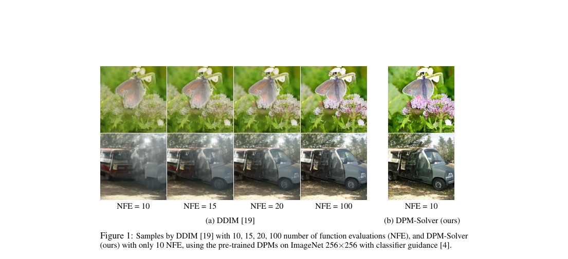
- ImageNet guided: strong few-step gains over DDIM at - NFE.
- Multiple datasets: reported - speedup over prior training-free samplers.
Table 1: FID on CIFAR-10 for different orders of RK methods and DPM-Solvers, varying the number of function evaluations (NFE).
| Plot | Methods shown | What it shows |
|---|---|---|
| CIFAR-10 (continuous) | ODE (DPM-Solver), ODE (RK45), SDE (Euler), SDE (Adaptive) | DPM-Solver reaches low FID in very few evaluations; SDE solvers need far more steps. |
| CIFAR-10 (discrete) | DPM-Solver, DDPM, Analytic-DDPM, DDIM, Analytic-DDIM, PNDM, GGDM | DPM-Solver dominates the low-NFE regime and approaches FID by steps. |
| CelebA (discrete) | DPM-Solver, DDPM, Analytic-DDPM, DDIM, Analytic-DDIM, PNDM, FastDPM, It^o-Taylor | DPM-Solver remains best or tied-best through the few-step region. |
Ablations
- Solver order: higher order helps most under tight NFE budgets.
- Step variable: uniform spacing in beats uniform spacing in .
- Adaptive schedule: preferred once NFE reaches about .
- Conditional sampling: the same solver remains effective with classifier guidance.
Method Strengths and Weaknesses
Strengths
- Exact treatment of the linear ODE part removes a major discretization source.
- Training-free drop-in sampler for both discrete-time and continuous-time DPMs.
- Third-order solver gives strong quality in - NFE.
- Works with classifier guidance and large-scale image models.
Weaknesses
- Quality still depends on the pretrained score model.
- Few-step gains come from deterministic ODE sampling, not stochastic correction.
- Higher-order variants need extra intermediate evaluations and bookkeeping.
- Theory covers convergence order, not full optimality under guidance mismatch.
Suggestions from the authors
- Study solvers of order with more intermediate points.
- Improve conditional sampling, especially under stronger guidance.
- Refine adaptive step-size control for better NFE-accuracy trade-offs.
- Extend dedicated solvers to broader diffusion formulations and schedules.
Links
Prior Papers
- @DenoisingDiffusionProbabilisticModels2020 — establishes the discrete-time diffusion formulation that DPM-Solver accelerates at sampling time.
- @DenoisingDiffusionImplicitModels2020 — provides the main deterministic few-step baseline that DPM-Solver substantially outperforms.
- @songScoreSDE2020 — gives the SDE/ODE unification that DPM-Solver specializes with a dedicated semi-linear solver.
- @nicholImprovedDDPM2021 — improves practical diffusion parameterizations and schedules that DPM-Solver can sample faster.
- @dhariwalDiffusionBeatGANs2021 — supplies the guided ImageNet diffusion models used to showcase few-step conditional sampling.
Further Papers
- @karrasEDM2022 — studies improved diffusion design choices and samplers in the same efficiency-quality space.
- @rombachLatentDiffusion2022 — makes diffusion sampling efficiency more consequential by moving generation into latent space.
- @peeblesDiT2022 — large diffusion transformers benefit directly from stronger few-step solvers.
- @songConsistencyModels2023 — pushes the same agenda further by collapsing diffusion sampling to very few steps.